Tutorial

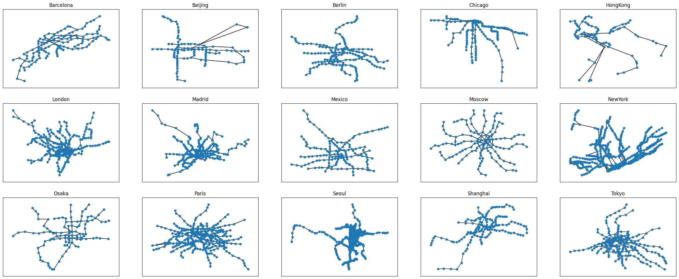
This tutorial presents some of the main features of the package. To illustrate the usage, we analyse a selection of subway networks of well known cities.

Before we start, let us import all necessary packages:

import matplotlib.pyplot as plt
import networkx as nx
import sys
import os
import numpy as np
from importlib import reload
from tabulate import tabulate
from IPython.display import HTML, display
import pandas as pd

import gdMetriX

We begin by loading the data from the datasets module, which provides access to the 'subways' dataset. The first time, this may take some time as the dataset has to be downloaded first. Afterwards, the data is cached locally.

subways = list(gdMetriX.iterate_dataset('subways'))

To see what we are dealing with, we first draw the graphs using matplotlib and networkX.

plt.figure(figsize=(30, 12))
i = 0
for name, graph in subways:
    # Setup the matplotlib axis
    ax = plt.subplot(3, 5, i + 1)
    ax.set_title(name)

    # Read the node positions from the graph
    pos = gdMetriX.get_node_positions(graph)

    # Draw on the axis using networkX
    nx.draw_networkx_edges(graph, pos, ax=ax)
    nx.draw_networkx_nodes(graph, pos, ax=ax, node_size=25)

    i += 1
plt.show()

Crossings

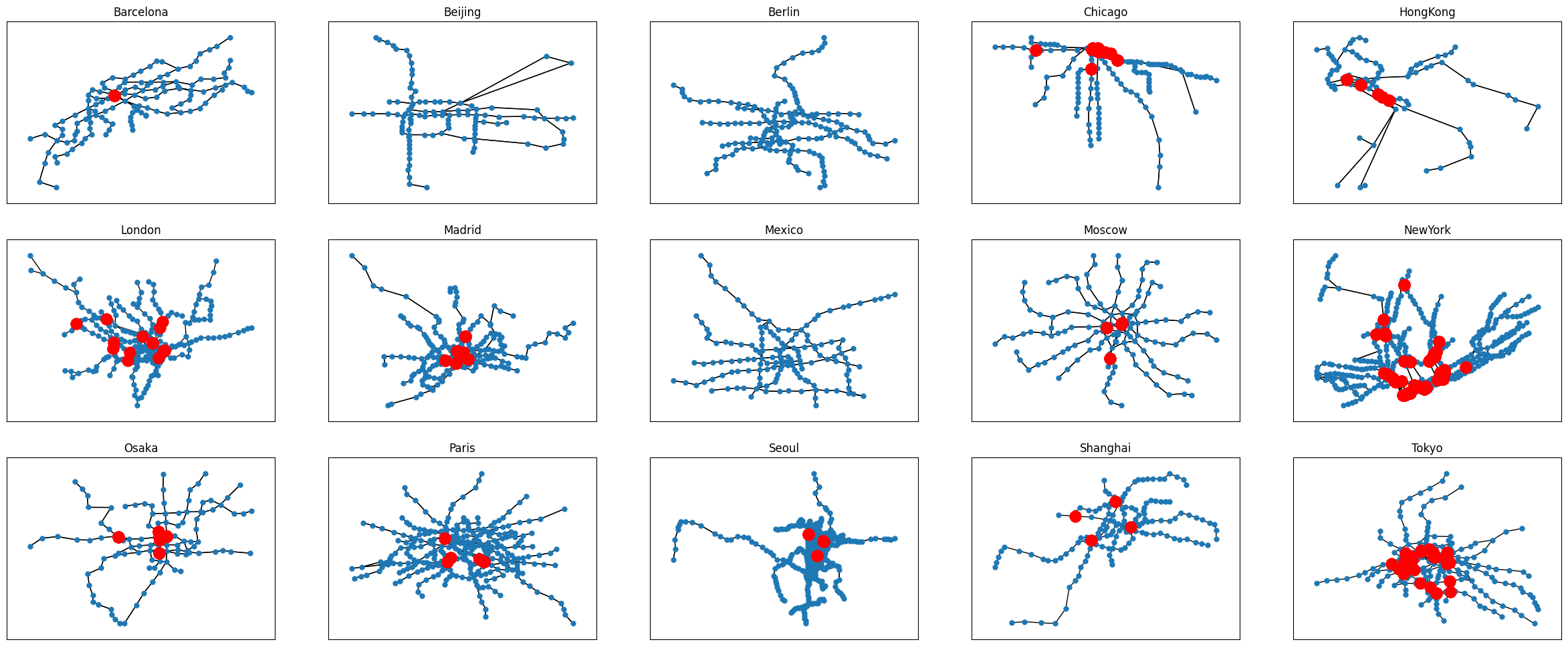
To begin with, we might want to determine where different lines cross each other without a transit station. To do so, we have to find all edge crossings, which can be achieved as follows.

plt.figure(figsize=(30, 12))
i = 0
for name, graph in subways:
    # Obtain a list of all crossings
    crossing_list = gdMetriX.get_crossings(graph)

    # Draw the graph first
    ax = plt.subplot(3, 5, i + 1)
    ax.set_title(name)
    pos = gdMetriX.get_node_positions(graph)
    nx.draw_networkx_edges(graph, pos, ax=ax)
    nx.draw_networkx_nodes(graph, pos, ax=ax, node_size=25)

    # Remove all crossing lines (we assume those to represent the same train track set)
    crossing_list = list(filter(lambda x: type(x.pos) is gdMetriX.crossingDataTypes.CrossingPoint, crossing_list))

    # Draw the crossings as red dots
    x_values = [point.pos.x for point in crossing_list]
    y_values = [point.pos.y for point in crossing_list]
    ax.plot(x_values, y_values, 'ro', ms=12)

    i += 1
plt.show()

Global attributes

Next, we create a list of global metrics for all subway networks. Refer to the documentation for a complete list of available metrics.

results = [
    ["Name", "n", "m", "Visual Symmetry", "Area", "Tight area", "Aspect ratio", "Height", "Width", "Center of mass", "Closest elements", "Closest points", "Concentration", "Gabriel ratio", "Homogeneity", "Horizontal balance", "Vertical Balance"]
]

for name, g in subways:
    graph_list = [name, g.order(), len(g.edges()), gdMetriX.visual_symmetry(g),
                  gdMetriX.area(g), gdMetriX.area_tight(g), gdMetriX.aspect_ratio(g),
                  gdMetriX.height(g), gdMetriX.width(g), gdMetriX.center_of_mass(g),
                  gdMetriX.closest_pair_of_elements(g)[2], gdMetriX.closet_pair_of_points(g)[2], gdMetriX.concentration(g),
                  gdMetriX.gabriel_ratio(g), gdMetriX.homogeneity(g), gdMetriX.horizontal_balance(g),
                  gdMetriX.vertical_balance(g)]

    results.append(graph_list)

df = pd.DataFrame(results)
display(HTML(df.to_html()))

	0	1	2	3	4	5	6	7	8	9	10	11	12	13	14	15	16	17
0	Name	n	m	Visual Symmetry	Area	Tight area	Aspect ratio	Bounding box	Height	Width	Center of mass	Closest elements	Closest points	Concentration	Gabriel ratio	Homogeneity	Horizontal balance	Vertical Balance
1	Barcelona	128	286	0.707802	0.0259	0.01177	0.554745	(41.343333, 2.0353131, 41.4632, 2.251389)	0.216076	0.119867	v(41.400485598437506,2.15647111171875)	0.000405	0.000424	0.535433	0.997946	1.0	0.3125	-0.125
2	Beijing	104	228	0.803643	0.120774	0.087965	0.467214	(39.8444, 116.171944, 40.081944, 116.6803702)	0.508426	0.237544	v(39.945206184615394,116.41587960384615)	0.00388	0.00388	0.592233	0.996345	0.999998	-0.307692	-0.326923
3	Berlin	170	364	0.760584	0.077929	0.051501	0.414477	(52.416111, 13.200278, 52.595833, 13.633889)	0.433611	0.179722	v(52.50868810588238,13.37589586470588)	0.001882	0.002515	0.597633	0.999084	1.0	-0.517647	0.094118
4	Chicago	141	298	0.723793	0.103609	0.053603	0.840046	(41.722596, -87.900876, 42.07379, -87.605857)	0.295019	0.351194	v(41.89951913333332,-87.68078670000001)	0.0	0.000931	0.65	0.997369	1.0	0.77305	-0.219858
5	HongKong	82	170	0.556229	0.086499	0.059596	0.805013	(22.264372, 113.936616, 22.528253, 114.264413)	0.327797	0.263881	v(22.349040353658538,114.15831179268294)	0.000472	0.002814	0.592593	0.994706	1.0	0.707317	-0.585366
6	London	266	308	0.694677	0.261322	0.178695	0.351455	(-0.611389, 51.402222, 0.2509, 51.705278)	0.303056	0.862289	v(-0.17365018421052628,51.53866646616539)	0.0	0.007593	0.633962	0.99743	1.0	-0.315789	0.067669
7	Madrid	208	480	0.829943	0.093491	0.049705	0.703776	(40.30359236, -3.811841853, 40.56010038, -3.447367855)	0.364474	0.256508	v(40.426940676971185,-3.67461855901923)	0.0	0.0	0.676329	0.998412	1.0	-0.644231	-0.163462
8	Mexico	147	328	0.877274	0.053625	0.038794	0.823691	(19.324427, -99.215899, 19.534595, -98.960745)	0.255154	0.210168	v(19.426182782312928,-99.12700180952378)	0.000278	0.004529	0.534247	0.998675	1.0	-0.605442	-0.088435
9	Moscow	134	312	0.89252	0.134583	0.095862	0.799659	(55.569722, 37.407778, 55.897778, 37.818023)	0.410245	0.328056	v(55.73970225373134,37.61470240298508)	0.00042	0.002095	0.458647	0.998057	0.999944	-0.059701	0.19403
10	NewYork	433	950	0.747255	0.090182	0.061338	0.844298	(40.576178, -74.031361, 40.903, -73.755426)	0.275935	0.326822	v(40.72945972979215,-73.93355020785226)	0.0	0.002191	0.608796	0.999123	1.0	-0.538106	-0.136259
11	Osaka	108	246	0.81138	0.036782	0.024961	0.884782	(34.556028, 135.4122, 34.75992, 135.5926)	0.1804	0.203892	v(34.67056508333334,135.51295197222223)	0.0	0.002163	0.514019	0.997507	0.999583	0.222222	0.296296
12	Paris	299	712	0.846795	0.038396	0.028243	0.719643	(2.228331, 48.77977215, 2.459317446, 48.946)	0.166228	0.230986	v(2.3437453335351166,48.860113404983295)	0.000001	0.002712	0.57047	0.998945	0.999999	-0.070234	0.043478
13	Seoul	392	874	0.798977	0.922816	0.538437	0.663896	(36.769628, 126.616708, 37.948611, 127.39943)	0.782722	1.178983	v(37.503326494897976,126.97862405612248)	0.000415	0.003272	0.785166	0.999378	1.0	-0.030612	0.790816
14	Shanghai	148	158	0.75015	0.152405	0.091711	0.917791	(31.0025, 121.224, 31.41, 121.598)	0.374	0.4075	v(31.228932081081084,121.46187795945949)	0.0	0.005099	0.605442	0.997096	1.0	0.628378	0.310811
15	Tokyo	217	262	0.861586	0.070981	0.04305	0.592517	(35.586859, 139.612885, 35.791938, 139.959)	0.346115	0.205079	v(35.69779647004608,139.74785092165905)	0.0	0.0	0.597222	0.997213	1.0	-0.62212	0.152074

<Figure size 100x100 with 0 Axes>

We can see, that Moscow has the most symmetric subway layout (according to the visual symmetry value of 0.89252), while Hong Kong has the most irregular layout (with a visual symmetry value of just 0.556229) . The London underground covers by far the most area, which more than 15 times larger than the smallest subway, Barcelona - according to the size of the tight area, which calculates area using the convex hull.

Edge- and nodewise parameters

Some properties are not global, but instead defined for each individual node, edge or crossing. We will illustrate how to analyse such local features. To do so, we are going to look at the distribution of edge lengths, which tells us how long the distance between stations is.

We begin by drawing some violin plots for the edge length distribution.

data = []
labels = []
for name, g in subways:
    pos = gdMetriX.get_node_positions(g)
    edge_lengths = [gdMetriX.euclidean_distance(pos[edge[0]], pos[edge[1]]) for edge in g.edges()]
    data.append(edge_lengths)
    labels.append(name)

data = sorted(data, key=lambda x: max(x), reverse=True)

fig, ax = plt.subplots()
fig.set_figheight(4)
fig.set_figwidth(16)
ax.set_xticks(np.arange(1, len(labels) + 1), labels=labels)
ax.violinplot(data)

plt.show()

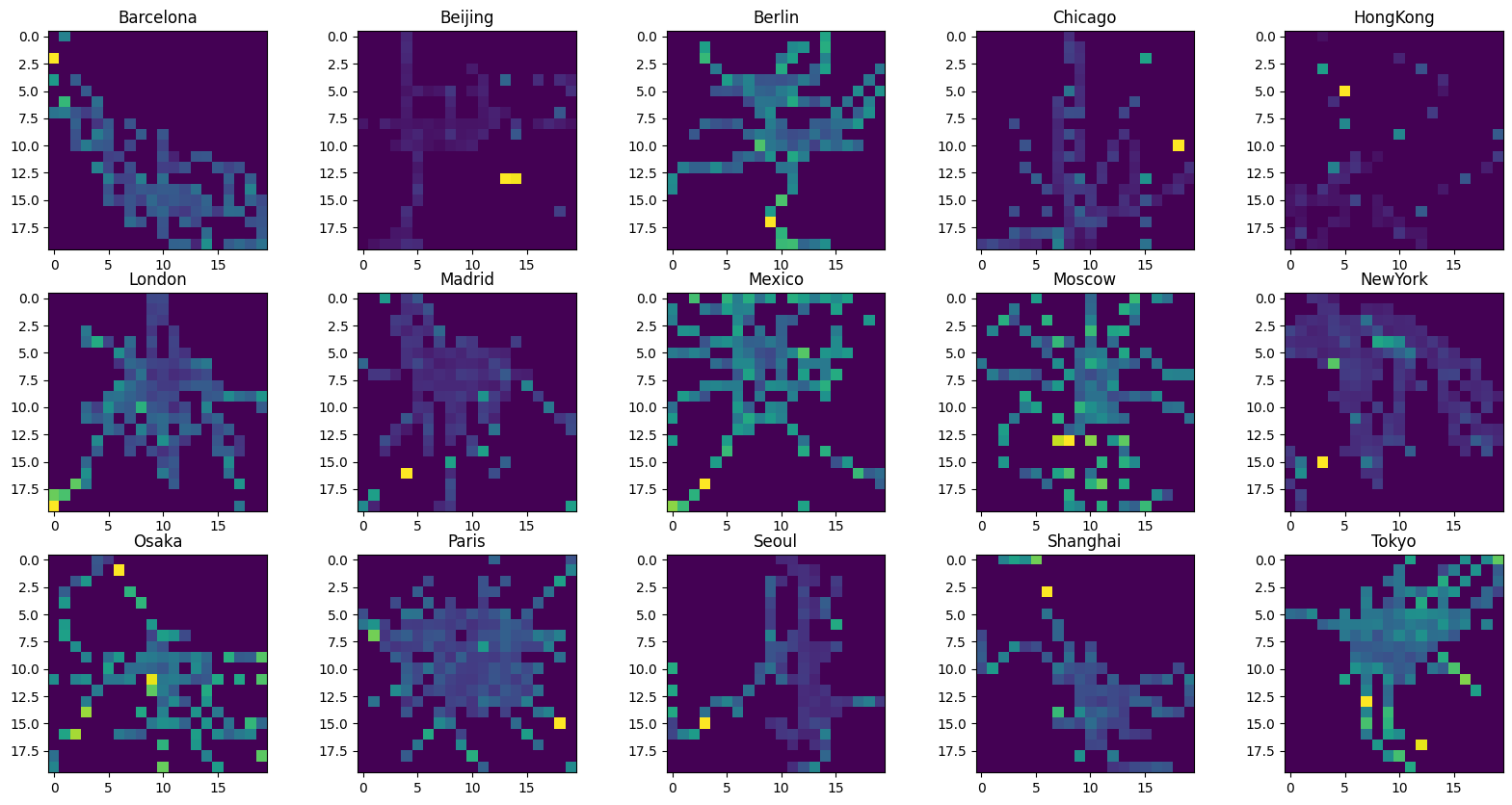
We can see that the distance between stations vary hugely. Let us plot the average edge length on a heatmap to spot densely populated areas using the heatmap function.

plt.figure(figsize=(20, 10))
i = 0
for name, g in subways:
    ax = plt.subplot(3, 5, i + 1)
    ax.set_title(name)

    pos = gdMetriX.get_node_positions(g)
    edge_lengths = [gdMetriX.euclidean_distance(pos[edge[0]], pos[edge[1]]) for edge in g.edges()]
    edge_pos = [gdMetriX.Vector.from_point(pos[edge[0]]).mid(gdMetriX.Vector.from_point(pos[edge[1]])) for edge in g.edges()]

    x_values = [x for x, y in pos.values()]
    y_values = [y for x, y in pos.values()]

    heatmap = gdMetriX.heatmap(g, edge_pos, edge_lengths, 20)
    ax.imshow(heatmap, cmap='viridis', interpolation='nearest')

    i+=1


plt.show()

For some cities, the average edge length seems to increase as one goes further away from the centre, however, for the most part, the edge lengths seem to be roughly evenly distributed. Maybe stations are still close along each subway line, but the distance between lines increases. Maybe we can detect a pattern when looking at the node density instead.

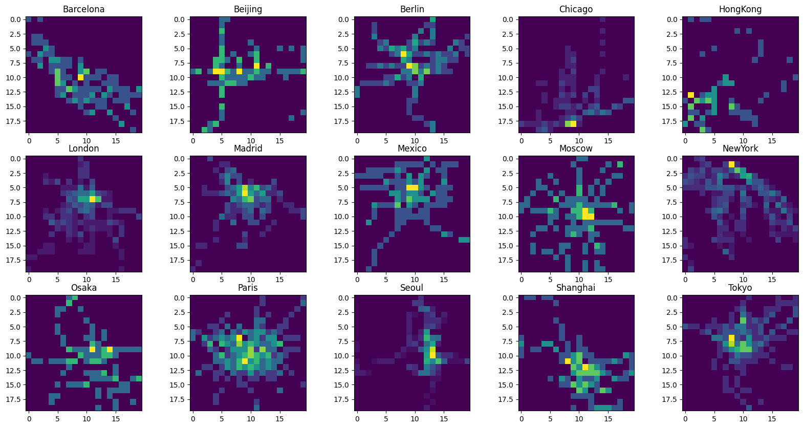
Instead of building the average of a value as for the edge length above, we simply want to count the number of vertices in each grid cell of the heatmap. To do so, we simply set average=False and supply None as the list of values.

plt.figure(figsize=(20, 10))
i = 0
for name, g in subways:
    ax = plt.subplot(3, 5, i + 1)
    ax.set_title(name)

    pos = [point for point in gdMetriX.get_node_positions(g).values()]
    heatmap = gdMetriX.heatmap(g, pos, None, 20, average=False)
    ax.imshow(heatmap, cmap='viridis', interpolation='nearest')

    i+=1

plt.show()

Seems that our hypothesis was correct. This time, the densely populated city centers are easily discernible.